Where Does a Vision Transformer Keep Its Sense of Geometry?

A self-supervised ViT can predict depth from a single image with no 3D supervision at all. That’s usually treated as one fact. A recent paper asks a sharper question: is that geometry sitting in a few clean directions the network can read out directly, or is it smeared across the whole feature space, waiting for a powerful decoder to untangle it?

Reading notes on Zhou et al., Understanding Geometric Representations in Self-Supervised Vision Transformers via Subspace Intervention · arXiv:2607.01987

Most evaluations of vision transformers stop at a single number: how well does a probe trained on top of frozen features perform? If it’s high, we say the model “understands” geometry. If it’s low, we shrug, maybe the information isn’t there, maybe it’s just hard to extract. This paper doesn’t accept that shrug. It opens the probe up and asks what it’s actually made of.

Is the geometry missing, tangled, or scattered?

Before touching the internals of a probe, the authors separate three different failure modes using three decoders of increasing power, applied to the same frozen features. A Linear probe reads geometry only if it’s already sitting in a straight line. A point-wise MLP adds a non-linearity but still looks at one patch at a time, the gap between Linear and MLP shows how much geometry is locally tangled. A DPT decoder adds full cross-patch aggregation, the gap between MLP and DPT shows how much is scattered across the image and only recoverable with global context.

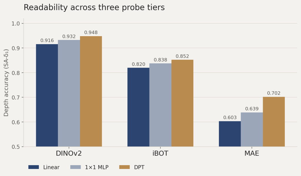
The pattern is stark. For DINOv2, the linear probe alone already gets most of the way there, the model arranges geometric information along a small set of straight, readable directions. For MAE, the linear number is much lower, and it’s the global decoder that closes most of the gap: the geometry is real, but spread across many patches at once. iBOT sits in between, consistent with its design as a hybrid of the two training styles.

This matters for anyone building lightweight decoders: a model that scores low on a probe might still contain the information, it might just need a wider receptive field to read it, not more capacity.

Opening up the probe itself

The more interesting move: a converged linear probe is just a weight matrix. The authors run SVD on it and keep only the top few directions, the ones the probe actually leans on, then project the original features onto that small subspace and re-run the same frozen probe. If performance barely drops, the geometry the probe cares about was living in a tiny corner of the feature space all along. Across every model tested, that’s exactly what happens: a random subspace of the same size collapses to noise, and so does the leftover residual once the top directions are removed. The explicit signal is concentrated, not diffuse, even in MAE, which spreads it wider than DINOv2 but still compresses well.

Where does the energy live, layer by layer?

Splitting the probe weights by which layer they came from shows how much each depth of the network contributes to the final geometric readout.

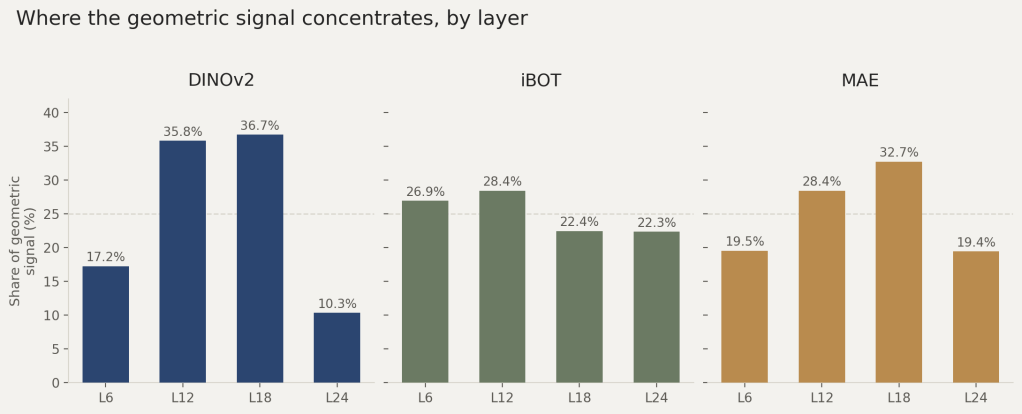
DINOv2 concentrates over 70% of its geometric signal in the two middle layers, then drops sharply by the final layer, a clear structural transition. iBOT and MAE stay close to an even split across all four depths, meaning their geometry is aggregated across the whole hierarchy rather than concentrated anywhere in particular.

What it adds up to

Three findings stack together. First, the training objective decides the format, not just the quality, of geometric representation, self-distillation aligns geometry into a compact, linearly readable code, while masked reconstruction keeps it dispersed to preserve the high-frequency detail pixel-level reconstruction needs. Second, whatever the format, the explicit part is highly compressible, even MAE’s more scattered signal saturates fast with a modest rank budget, a real hint for anyone designing dense prediction heads. Third, geometry is not a terminal-layer property: for DINOv2, geometric precision peaks mid-network and fades by the final layers, right as semantic segmentation is still climbing, reading only the last layer misses where geometry is most available.

This is a useful companion to questions about spatial relations rather than raw depth. If depth sits in a compact subspace at intermediate layers, it’s worth checking whether relational cues, left/right, inside/outside, containment, show the same pattern, or need the global aggregation that MAE-style geometry depends on. The subspace intervention method itself is directly reusable as a diagnostic tool for that question, independent of the target task.

Where to be careful

The authors are upfront about the limits. The method isolates linear, explicit structure well, but can’t unpick features that are genuinely non-linearly entangled. The evaluation depends on datasets with aligned depth, normals, and semantics, which restricts generalization beyond indoor scenes like NYU Depth V2, and the largest backbone tested is ViT-Large rather than ViT-Giant.